In this article we explore using one of the coolest data sets for the upland hunter, the Cornell eBird Database. The jig is up, I’ve been using the maps for a while now, and when I posted about it on Social Media last year I saw a couple other upland bird hunting personalities, Jorge and Rob, admitted to also using them for a little informed scouting. You might be asking, am I not scared that revealing this data source will somehow cause a mass influx of hunters to choice spots? Not really, and here’s why: dedication.
Acquiring Your Custom Data Set
In order to get access to the dataset itself you need to first break the barrier of asking the Cornell Ornithology Lab, which isn’t that big of a deal. Next, you need to have invested some time in making some Hunting Maps for Lunatics — but more importantly, now you need the spare time to pour over 30 gigabytes of bird sighting data. What in the what?! I learned the hard way that when a birder goes out with their checklist and goes to observe a given area, they record the entire checklist in this data, meaning that it’s Comma Separated Values several hundred or thousand entries wide by an entire year worth of observations.
I downloaded the entire data set for all birds, which may not be advisable to you unless you have a bunch of hard drive space and access to a Linux computer for some data crunching. Linux?! I thought this was a hunting and fishing blog?! In time, padawan. In Windows 10 you can use the Windows Subsystem for Linux (WSL) to get done what we’re looking to here without too much investment, if you have a Mac you’re in luck since we’re just using a few native commands to select the data set we actually want from the larger one.
Note: The license for the eBird dataset prohibits me from further disseminating it, and I’d like to continue having access. It’s also giant in size, so while I’d like to host a 30GB tarball on my website it’s just not feasible right now. So I can give you instructions on where and how to get it, and manipulate it similarly to what I’ve done for your own benefit.
A Little Command-line Fu Required
On Windows once WSL is installed with the distribution of your choice, navigate to where you downloaded the dataset and launch a Linux terminal, or on Mac just launch a terminal and cd to the directory where you downloaded the file. In your new terminal window in your download directory we’re going to untar the file, called a tarball. Ensure that we have enough elbow room as you’re going to need at least 30GB of free space plus any processing you’re going to want to do. In that terminal window we’re going to untar the file with the following command:
| tar -xvf ebird_reference_dataset_v2016_western_hemisphere.tar |
It may take some time as the file is quite large, get some coffee and come back in 20 minutes or so. Navigate inside the folder that is generated with the cd (change directories) command and eventually you’ll come upon a folder full of years, that a checklist for each year the data has been observed, digitized, and compiled. Let’s cd into 2016 for the most recent data on record. Inside that folder you have two files, checklists.csv.gz and checklists-covariates.csv.gz, our target is checklists.csv.gz, so lets run gunzip checklists.csv.gz in our terminal window. Gunzip will unzil the gz file, and it is installed by default on nearly all Linux variants and MacOS. This will take a little bit of time as the file expands, and you’ll be left with, yet another folder with checklists.csv inside. It may seem trivial at this point where you say “Alex, I can open a csv file inside of Excel! This isn’t that big of a deal!” Accurate, you totally can, but at 29.1GB for just one text file, it’s likely your computer will hang until the next woodcock migration before it loads the file. We’re going to use some system commands to manipulate the file to our own devices before we do anything with mapping. To get an idea of how many birds are counted let’s run the following command:
| head -n 1 checklists.csv |
This will take the top line of the file and display it for you, this is just the header of the file, the same as it would be across an Excel spreadsheet. You’ll notice it would be a couple hundred lines long. That’s just ridiculous to be able to crunch through in a reasonable amount of time. Here’s where I’d like to ask you to pause and think about what we’re looking to do. Do you have a target set of game birds you’re looking to do some research on? Do you have a target state you’d like to hunt? Is this more work than you’re interested in for the sake of research? Think about your bucket list hunts, and whether this data set will even help you
In the previous post I made mention that I’m pretty keenly interested in Ptarmigan hunting in Colorado. It’s an odd bird that’s been gaining in social media popularity and is extremely niche amongst bird hunters to begin with. Let’s use that as our exemplar here. To create the file we’re interested in, with only Colorado ptarmigan data we run the following two commands:
| head -n 1 checklists.csv | awk -F”,” ‘{ print $1″,”$2″,”$3″,”$4″,”$5″,”$6″,”$7″,”$8″,”$9″,”$10″,”$11″,”$12″,”$13″,”$2108″,”$2109″,”$2110″,”$2111}’ | grep -i “Colorado” > CO_ptar.csv awk -F”,” ‘{ print $1″,”$2″,”$3″,”$4″,”$5″,”$6″,”$7″,”$8″,”$9″,”$10″,”$11″,”$12″,”$13″,”$2108″,”$2109″,”$2110″,”$2111}’ checklists.csv | grep -i “Colorado” >> CO_ptar.csv |
The first command creates the header, we know we want data related to the time and date of the bird survey, the location data including LAT and LON data, the County, the State, and the count of actual birds. Awk takes the data and pares it down to only the fields we want, and the carrots write a new file, a single carrot to redirect to a new file, double to append to it, so we’re writing the header, and then appending the data we want with the same fields. Here we select every type of ptarmigan even though only the white tailed ptarmigan (Lagopus leucura) lives in the state if you were interested in Canada or parts of Alaska the other fields would be populated. Of note, all of the bird names in the data are in Latin, so fire up some Wikipedia to figure out what birds you’re interested in. I’ve included some below for reference. Looking for another particular bird and want to modify the commands above to suit? Find what field it’s in by running the following command, and modify the two commands above to replace ptarmigan data with that of your own bucketlist bird!
| head -n 1 checklists.csv | awk -F”,” ‘{for(i=1;i<=NF;i++){if ($i ~ /Lagopus/){print i}}}’ |
The output of this will tell you which columns match the search enclosed in the regular expression (bounded by //). Your output will look like this:
| 2109 2110 2111 |
On to the Maps!
Easy, right? So now we have a new file, CO_ptar.csv — how do we use it? Put the file somewhere it won’t disappear and load up our map we created before.
Open up that project you saved before, and now let’s go to Layers -> Add Layer -> Add Delimited Text Layer like so.

You’ll be presented with a dialog where you have a couple different fields we’ll need to configure before the data is useful. Make sure the File Format is Comma Separated Value (CSV), and select your CO_ptar.csv that we created earlier. Because of the work we did earlier to create the header and the data, the dialog auto-populates Longitude and Latitude, otherwise you’d have to manually select which fields were which — if dealing with a different data set this can be troublesome and time consuming. Click Add to add the data to your project aaaaaand nothing will happen.
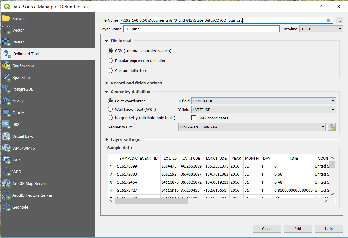
So what gives? You just went through all of that data crunching for nothing to happen? Well, QGis doesn’t necessarily know how to represent the data we just added to the project, so we have to do just a little more manipulation to make it useful, and visible.
Find the newly added Layer, right click and go to Properties. On the left hand menu select Source Fields, notice those purple lines on my screenshot? We’re going to create those fields for use later.
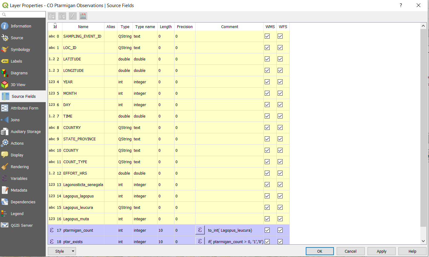
At the top of the dialog there are four buttons, clicking the rightmost button (Field Calculator) allows us to create a new field that is based on existing data. We’re going to create two additional fields here based on current data that will affect how our data can be displayed on the map and overcome some wierdness with QGis. Because of the way the data are collected for the eBird observation sometimes there are partial birds marked because there are observation hours and birds calculated on each visit. For this reason we’re going to create the field ptar_count which will give us an integer of ptarmigan found in the area. So in the Output Field Name, type ptar_count and in the Expression editor type the following:
| to_int( Lagopus_leucura) |
And click Ok. The field will display as purple. If you’re playing around trying to see other expressions that would be useful in your data analysis, there’s an Output Preview right underneath the expression editor that will show a preview of the expression on the column of choice.
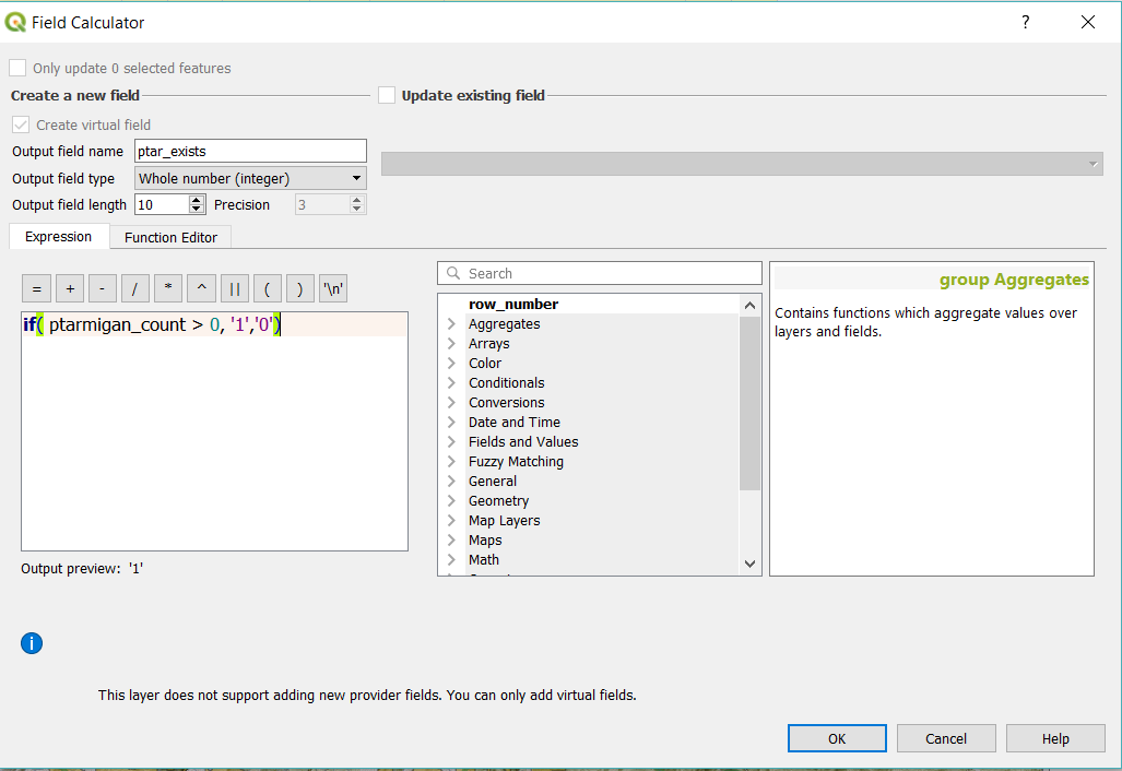
Now let’s repeat the process and make a column called ptar_exists. This will be a simpler yay/nay as to whether a ptarmigan has been seen in that area. Remember when I had you awk the checklists.csv? There still seemed to be a ton of data there right? That’s because a ptarmigan is on everyone’s checklist whether they’re in the forests, mountains, or desert. All we really did was choose a column and make sure we only selected data from Colorado. If we displayed everything here, you’d get the false impression ptarmigan were everywhere including downtown Denver.
For the ptar_exists column we’ll use the following expression:
| if( ptar_count > 0, ‘1’,’0′) |
Basically this uses programming if-logic in order to set a one or a zero based off of whether the integer ptarmigan count is greater than zero. We’ll use this as a display filter later. Click OK and add this one to the fields.
Now we have some derivative data from the study data we can use for mapping purposes. Let’s put this to use, shall we? Go to the Symbology Tab still in the Layer Properties Dialog and select “Graduated” from the drop down and then for the column use ptar_count. Select a Color Ramp from the drop down, I like Orange to Red to stand out against our existing sepia toned map. Set the mode to Equal Interval and then Click Classify. This will classify your data and assign colors along the gradient to each classification. For the first classification, make sure you set the minimum value to 1 instead of zero, and click OK.
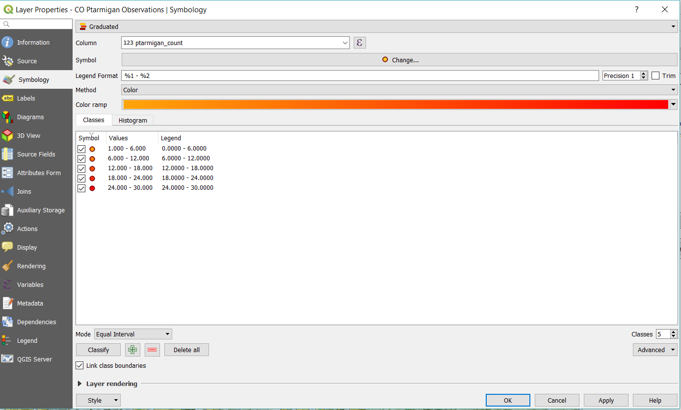
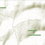
Now that you’ve added graduated labels and filtered them in one fell swoop, you’ll see dots appear on the map in the points where ptarmigan were observed in Colorado, graduated by color such that the red dots had the most total observations, tight clusters indicate multiple observations.
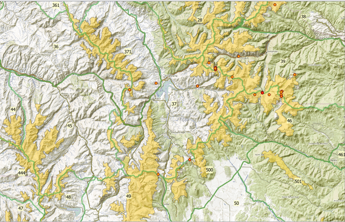
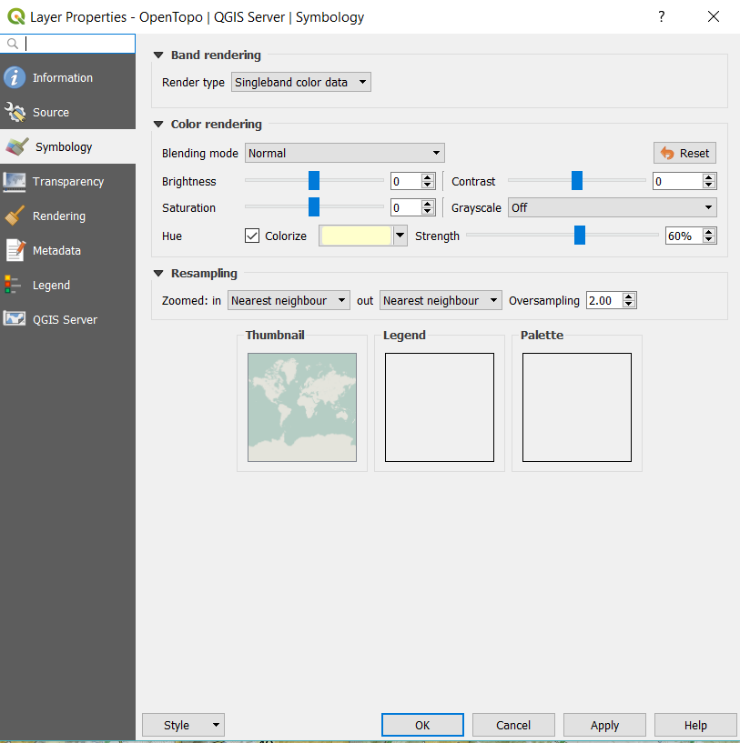
How did I get the map to look like the above? I added the OpenTopo layer I made mention of in the last post, and blanketed the layer with a yellowed overtone with some transparency, 60% opacity by right clicking the Layer and going to Properties.
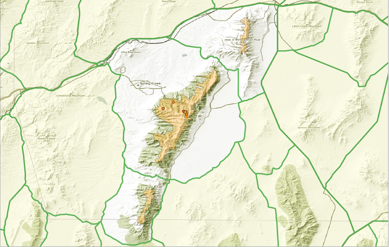
Pretty cool, right? Now you have the basics to adding one of the more complicated outdoor datasets for birds. This could be a boon to Chukar chasers, Pheasant Fanatics, Grouse goons, and the psychopaths chasing Himalayan Snowcock in Nevada.
Latin Binomial Names of Game Birds
| Scaled Quail – Callipepla squamata Gambel Quail – Callipepla gambelii Bobwhite Quail – Colinus virginianus Himilayan Snowcock – Tetraogallus himalayensis Ringneck Pheasant – Phasianus colchicus Chuckar – Alectoris chukar Sage Grouse (lesser and greater)- Centrocercus minimus and Centrocercus urophasianus Sharp Tailed Grouse – Tympanuchus phasianellus Prairie Chicken (Lesser and Greater) -Tympanuchus cupido, Tympanuchus pallidicinctus |


[…] « Previous Story […]